Introduction to the Data in PRECISION.seq
Intro_Data.RmdMicroRNA (miRNA) sequencing data were collected for two subtypes of soft tissue sarcoma: myxofibrosarcoma (MXF) and pleomorphic malignant fibrous histiocytoma (PMFH). 27 MXF samples and 27 PMFH samples were collected from newly diagnosed untreated tumors at Memorial Sloan Kettering Cancer Center between 2002 and 2012. These tumor samples were sequenced twice: once with uniform handling and balanced sample-to-library-assignment to minimize data artifacts due to experimental handling and avoid their confounding with sample group (that is, tumor subtype); and a second time without, which resulted in excessive artifacts due to handling. The first dataset can be used to assess microRNAs’ differential expression status, serving as a benchmark; the second dataset can be used to test normalization methods against the benchmark. These two datsets are named as data.benchmark and data.test in this package.
We show (1) how to examine the overall distribution of each dataset, (2) how to perform differential expression analysis for each data set and compare the results between the two, and (3) how to create additional paired data sets based on a novel data permutation algorithm and analyze them.
Benchmark Data Analysis
Overall Data Distribution
We examine the overall distribution of the benchmark data (as log2 transformed read counts) using sample-specific boxplots.
benchmark.log <- log2(data.benchmark + 1)
boxplot(benchmark.log,
        col = ifelse(grepl("MXF", colnames(benchmark.log)),
                     rainbow(2)[1], rainbow(2)[2]),
        ylab = "Log2 Count", ylim = c(0, 20),
        xaxt = "n", outline = FALSE)
legend("topright",c("MXF", "PMFH"), bty = "n",
       pch = "x", cex = 1, col = c(rainbow(2)[1], rainbow(2)[2]))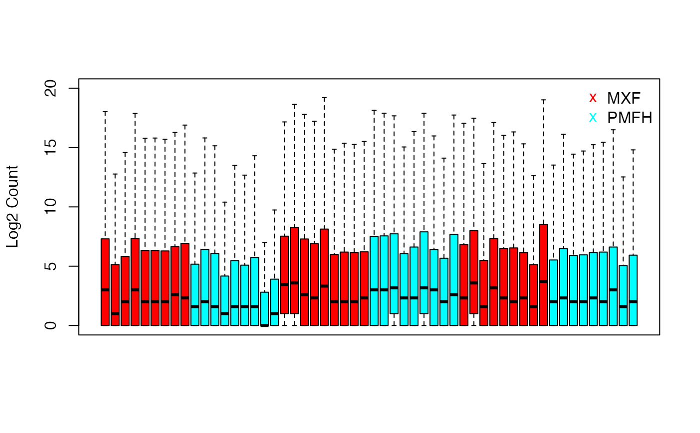
Differential Expression Analysis
We assess evidence for differential expression in the benchmark data using the voom-limma method. The analysis results are displayed with the volcano plot and the scatter plot of group mean difference versus group mean average. Red dots indicate the microRNAs that are significantly differentially expressed (\(p < 0.01\)).
benchmark.voom <- DE.voom(RC = data.benchmark, groups = data.group, Pval = 0.01)
DE.bench <- benchmark.voom$id.list
benchmark.voom.dat <- data.frame(dm = benchmark.voom$log2.FC,
                                 p.value = benchmark.voom$p.val)
mask <- with(benchmark.voom.dat, p.value < .01)
cols <- ifelse(mask,"red", "black")
with(benchmark.voom.dat, plot(dm, -log10(p.value), cex = .5, pch = 16,
                          col = cols, xlim = c(-3.6, 3.6),
                          ylim = c(0, 6),
                          xlab = "Mean Difference: PMFH - MXF"))
abline(h = 2, lty = 2)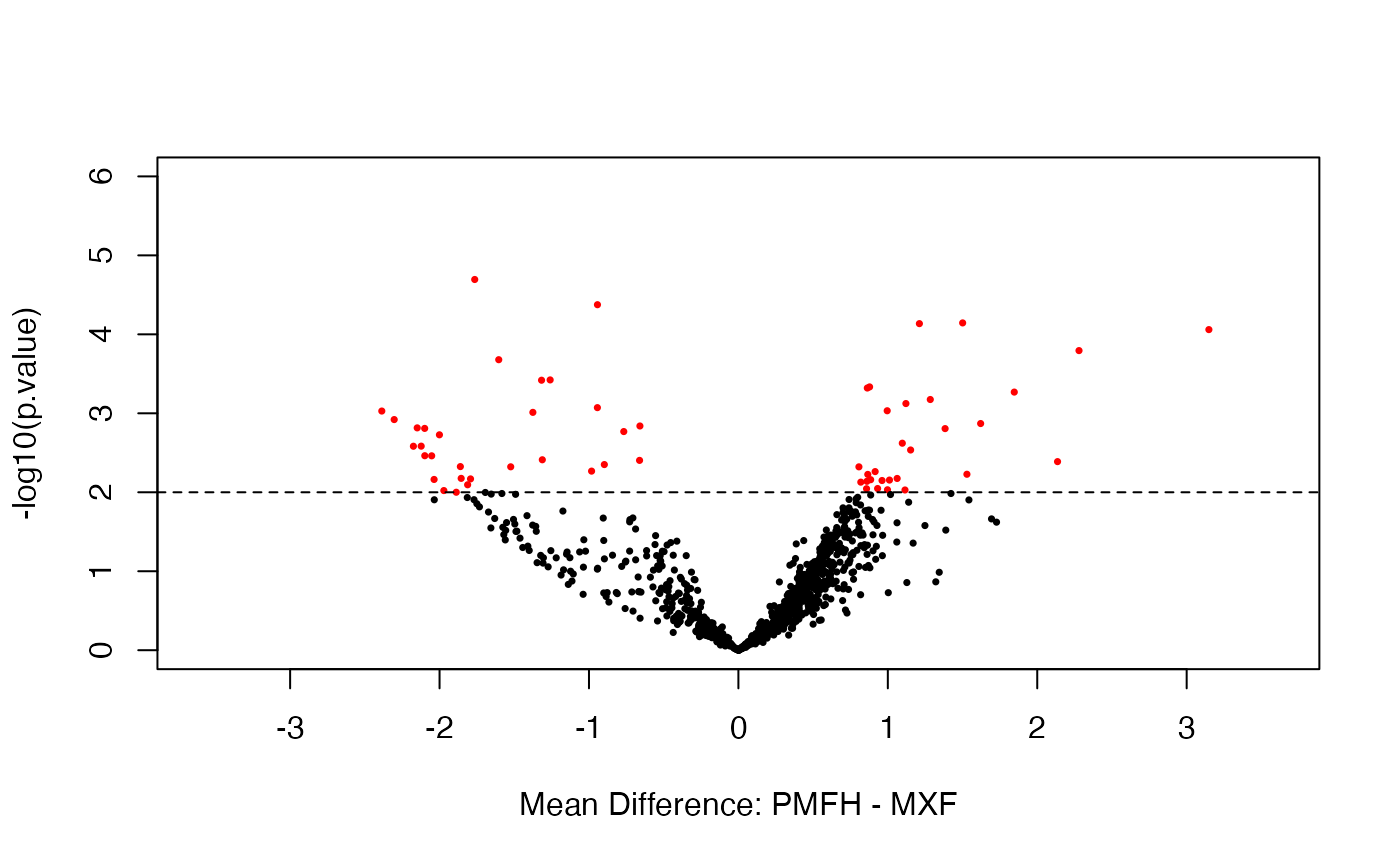
cols <- ifelse(rownames(benchmark.log) %in% DE.bench, "red", "black")
plot(rowMeans(benchmark.log),
     apply(benchmark.log[,grepl("MXF", colnames(benchmark.log))], 1, mean) -
       apply(benchmark.log[,grepl("PMFH", colnames(benchmark.log))], 1, mean),
     pch = 16, cex = 0.5, col = cols,
     xlab = "Group Mean Average of Log2 Count",
     ylab = "Group Mean Difference of Log2 Count",
     main = "")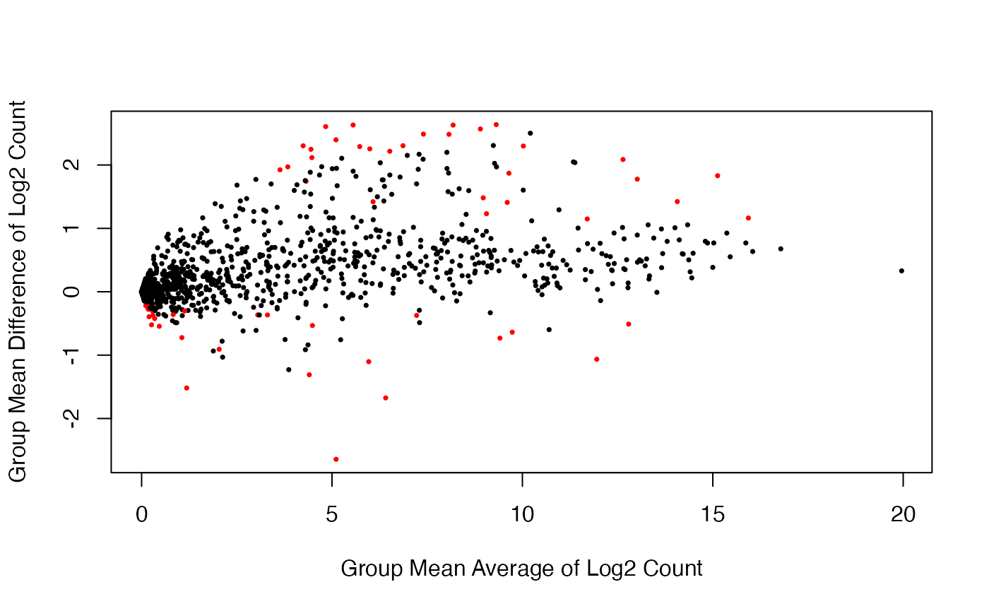
Test Data Analysis
Overall Data Distribution
We examine the overall distribution of the test data (as log2 transformed read counts) using sample-specific boxplots.
test.log <- log2(data.test + 1)
boxplot(test.log,
        col = ifelse(grepl("MXF", colnames(benchmark.log)),
                     rainbow(2)[1], rainbow(2)[2]),
        xaxt = "n", outline = FALSE, ylim = c(0, 20))
legend("topleft",c("MXF", "PMFH"), bty = "n",
       pch = "x", cex = 1, col = c(rainbow(2)[1], rainbow(2)[2]))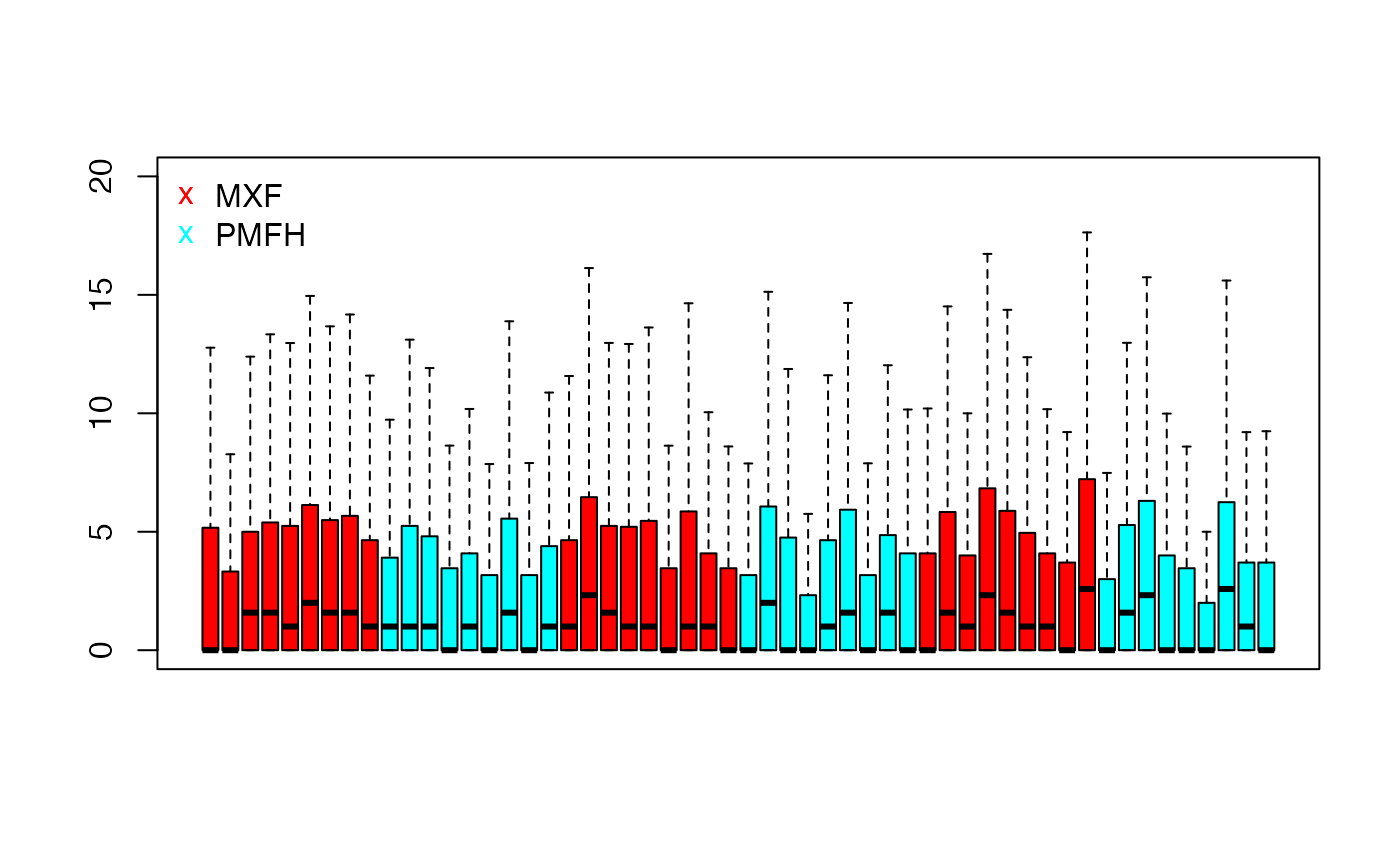
Differential Expression Analysis
We assess evidence for differential expression in the test data using the voom-limma method (without depth normalization). The analysis results are displayed with the volcano plot and the scatter plot of group mean difference versus group mean average. Red dots indicate the microRNAs that are significantly differentially expressed (\(p < 0.01\)).
test.voom <- DE.voom(RC = data.test, groups = data.group, Pval = 0.01)
test.voom.dat <- data.frame(dm = test.voom$log2.FC,
                            p.value = test.voom$p.val)
mask <- with(test.voom.dat, p.value < .01)
cols <- ifelse(mask,"red", "black")
with(test.voom.dat, plot(dm, -log10(p.value), cex = .5, pch = 16,
                         ylim = c(0, 6), xlim = c(-3.6, 3.6),
                         col = cols, xlab = "Mean Difference: PMFH - MXF"))
abline(h = 2, lty = 2)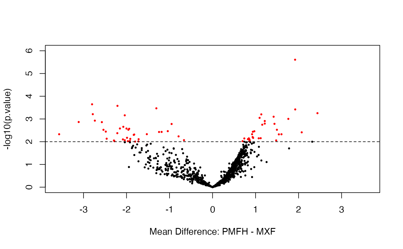
Comparison of Differential Expression Status Between Benchmark Data and Test Data
Significance of differential expression is claimed using a p-value cutoff of 0.01 for both the benchmark data and the test data. They are compared with each other using the Venn diagram.
pval.bench.test <- data.frame(cbind(bench.pval = benchmark.voom$p.val,
                                    test.pval = test.voom$p.val[names(benchmark.voom$p.val)]))
attach(pval.bench.test)
bench.sig <- (bench.pval < 0.01)
test.sig <- (test.pval < 0.01)
venn2 <- cbind(bench.sig, test.sig)
vennDiagram(vennCounts(venn2),
            names = c("Benchmark", "Test"),
            cex = 1.5, counts.col = rainbow(1))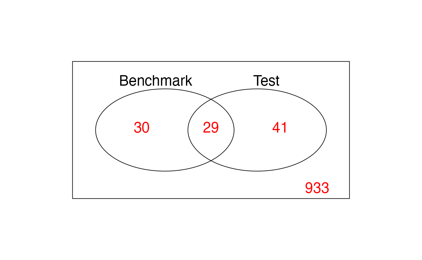
Comparison of Estimated Group Means Between Benchmark Data and Test Data
Scatterplot for the estimated group means for MXF and PMFH between benchmark data and test data.
benchmark.log.MXF.mean <- rowMeans(benchmark.log[, grepl("MXF", colnames(benchmark.log))])
plot(benchmark.log.MXF.mean,
     rowMeans(test.log[,grepl("MXF", colnames(test.log))]), pch = 16, cex = 0.5,
     xlab = "Group Mean Average of Log2 Count in Benchmark",
     ylab = "Group Mean Average of Log2 Count in Test",
     main = "MXF", xlim = c(0, 20), ylim = c(0, 20))
abline(0,1)
benchmark.log.PMFH.mean <- rowMeans(benchmark.log[, grepl("PMFH", colnames(benchmark.log))])
plot(benchmark.log.PMFH.mean,
     rowMeans(test.log[,grepl("PMFH", colnames(test.log))]), pch = 16, cex = 0.5,
     xlab = "Group Mean Average of Log2 Count in Benchmark",
     ylab = "Group Mean AVerage of Log2 Count in Test",
     main = "PMFH", xlim = c(0, 20), ylim = c(0, 20))
abline(0,1)
Simulation
We use simulated.data() function to generate additional pairs of data sets by permuting the paired data sets to achieve a pre-specified proportion and magnitude of differential expression. As an example, we show how to generate data sets with the proportion of differential expression around 0.02 (more specifically, in the range of 0.0175 and 0.0225) and the median of mean differences (for log2 counts) around 0 (more specifically, in the range of -0.5 and 0.5).
simulated <- simulated.data(proportion = c(0.0175, 0.0225), median = c(-0.5, 0.5), numsets = 100)

head(simulated[[1]]$simulated_benchmark)[,1:5]
#>                  D17    D7   D19    E3     E5
#> hsa-let-7a-2*      4     2     2     5     11
#> hsa-let-7a(3)  61589 30934 40506 69704 268842
#> hsa-let-7a*(2)   436   216   196   353   1517
#> hsa-let-7b     29023  8395 25772 17920  77765
#> hsa-let-7b*      125    50   106    92    607
#> hsa-let-7c      9774  5633 17112 13838  65477
head(simulated[[1]]$simulated_test)[,1:5]
#>                  D17    D7   D19    E3     E5
#> hsa-let-7a-2*      1     2     0     0      2
#> hsa-let-7a(3)  53958 89726 60273 21107 253696
#> hsa-let-7a*(2)   113   368   157   137   1162
#> hsa-let-7b     15832 17546 25624  4744  93419
#> hsa-let-7b*       32    48    73    15    258
#> hsa-let-7c      8156 11921 16656  4445  71733